Counting the number of finite rings
Introduction
Inspired by the attempt at counting abelian groups, we can attempt to look at counting other algebraic structures, this time for rings.
Our recipe was:
- Write down a multiplicative function for our counting problem.
- Write down and simplify the Dirichlet generating function for said function.
- Use the tools of complex analysis to get asymptotics.
In general, our counting problems won’t follow some of the constraints here, and we’ll have to adapt accordingly.
For instance, it is nice if a function is multiplicative or completely multiplicative, but not necessary for the Dirichlet generating function. It just could make it easier to find a nice form for the function.
For 2), we need our counting function \(f(n)\) to grow at most polynomially in \(n\). Otherwise, our Dirichlet generating function will not converge anywhere in the complex plane, meaning we can’t use any of our tools. We will have to resort to other counting methods.
We will look at a few problems on asymptotics on counting rings \(R\), showing how we may have to use other tools for estimation. And then we will look at a problem that is very similar to our abelian group counting problem, using the same tools as before.
Counting Rings
A ring \(R\) is a set \(R\) with two operations \(\times\) and \(+\), satisfying the following axioms:
- \(R\) is an abelian group under \(+\)
- \(R\) is closed under \(\times\), and \(\times\) is associative.
- \(R\) satisfies left and right distributivity:
- \(a \times (b + c) = (a \times b) + (b \times c), \, \forall a, b, c \in R\)
- \((b + c) \times a = (b \times a) + (c \times a), \, \forall a, b, c \in R\)
If \(R\) contains a multiplicative identity \(1\), then this is a ring with unity. Likewise, if \(\times\) is commutative, then this is a commutative ring.
Let \(r(n)\) be the number of rings (not necessarily with identity) with \(n\) elements. Let \(n = st\) where \((s, t) = 1\), and \(R_m = \{x \in R | mx = 0\}\), where \(m\) is a natural numbers. Then \(R_m\) is an ideal of our original ring \(R\), and in particular \(R_s\) and \(R_t\) are both ideals of \(R\)1
1 These are double-sided ideals.
Now if \(z \in R_s \cap R_t\), then \(sz = tz = 0\). As \((s, t) = 1\), by Bezout’s theorem we have \(as + bt = 1\), for some \(a, b \in \mathbb{Z}\). Thus \(z = 1z = asz + btz = 0\), so \(R_s \cap R_t = \{0\}\). Finally, if \(x \in R\), \(x = (1)x = asx + btx, \, asx \in R_t\) and \(btx \in R_s\) (since \(n = st\)), so that makes \(R = R_s \times R_t\). Thus, for \(n = \prod_{i=1}^m p_i^{k_i}\) we have \(R = \prod_{i=1}^m R_{p_i^{k_i}}\), \(|R_{p_i^{k_i}}| = p_i^{k_i}\).
If we constrain our ring to be commutative, than \(R_s, R_t\) will also inherit commutativity, and so we get an analagous decomposition.
If our ring has a multiplicative identity \(1\), then \(1 = as1 + bt1\). Note \(1^2 = (as1 + bt1)^2 = (as1)^2 + (bt1)^2 = 1\). Hence \((as1)^2 = as1, \, (bt1)^2 = bt1\). We have then found idempotents \(e_1 \in R_s\) and \(e_2 \in R_t\) such that \(e_i^2 = e_i,\, e_1 e_2 = e_2 e_1 = 0, e_1 + e_2 = 1\).
Thus if \(z \in R_s, z = z(1) = z(e_1 + e_2) = z(e_1)\), so \(e_1\) acts like a right identity in \(R_s\). Likewise, \(e_1\) acts like a left identity and \(e_2\) is a multiplicative identity in \(R_t\). Thus our factorization reduces down to rings with identity.
Let \(r^*(n)\) be the number of rings with identity, \(c(n)\) the number of commutative rings and \(c^*(n)\) number of commutative rings with identity.
Then we have just shown \(r, r^*, c, c^*\) are all multiplicative, and so we will need to study \(f(p^k)\).
In fact we have the following2:
2 This is due to a result by Blackburn and McLean See here for details.
| Function | Asymptotics |
|---|---|
| \(r(p^k)\) | \(p^{\frac{4}{27}k^3 + O(k^{2.5})}\) |
| \(r^*(p^k)\) | \(p^{\frac{4}{27}k^3 + O(k^{2.5})}\) |
| \(c(p^k)\) | \(p^{\frac{2}{27}k^3 + O(k^{2.5})}\) |
| \(c^*(p^k)\) | \(p^{\frac{2}{27}k^3 + O(k^{2.5})}\) |
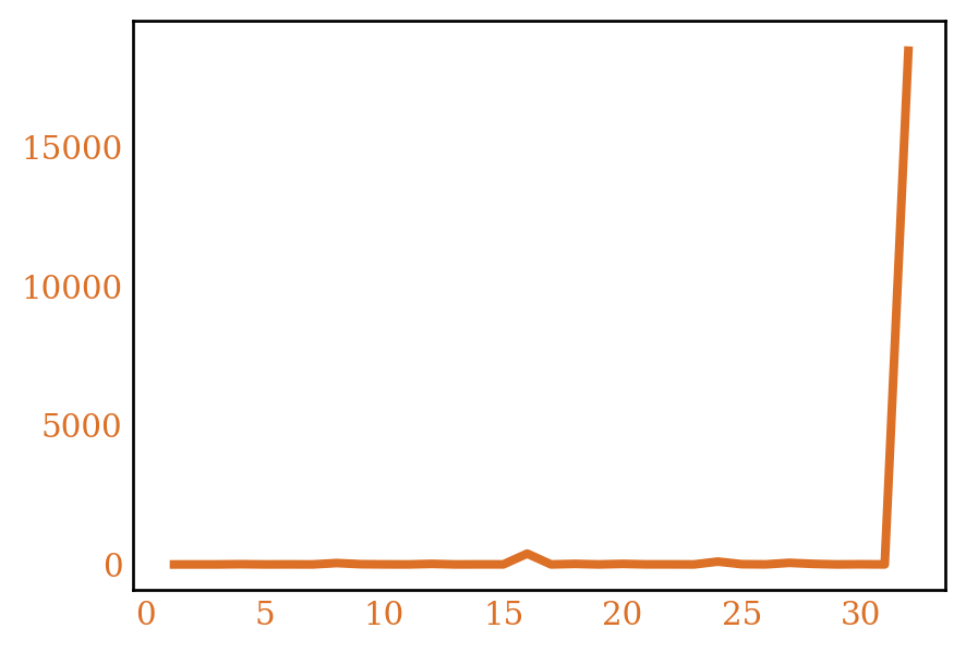
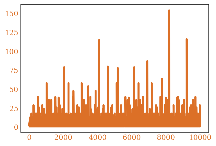
We can see some plots for these functions in Figure 13
3 \(r(32) > 18500\), but the actual value isn’t known. The value is listed in the plot, mostly to show how dramatically this function increases at powers of 2.
One would expect that the number of (commutative) rings (with identity) would grow super-polynomially based on this. Because of this, we can’t analyze the growth rate directly with Dirichlet generating functions since they wouldn’t converge anywhere.
For simplification, we will look at a multiplicative function \(f(p^k) = p^{c k^3}\), for some \(c > 0\). Understanding the asymptotics of this, will give some understanding of the asymptotics for all these functions.
We’ll investigate both \(\frac{1}{x}\sum_{n \le x} f(n)\) and \(\frac{1}{x}\sum_{n \le x} \log f(n)\).
\(\frac{1}{x}\sum_{n \le x} f(n)\)
Looking at \(\frac{1}{x}\sum_{n \le x} f(n)\), we can investigate the size of the largest term. If \(n = 2^{\lfloor \log_2 x \rfloor}\), then \(f(n) = 2^{c(\lfloor \log_2 x \rfloor)^3} \le e^{c(\log 2)^{-2}(\log x)^3}\). For \(x\) large enough this should be the largest term.
This is because if we look at \(m^{c(\lfloor \log_m x \rfloor)^3}\), it can be shown that this is a decreasing function so will be maximized over primes at \(m=2\). We can then show that once we look at composite numbers, for \(x\) large enough, as well this function is maximized at a power of \(2\) (which is left for the reader).
This then gives a rough bound for \(e^{c(\lfloor \log_2 x \rfloor)^3 - \log x} \le \frac{1}{x}\sum_{n \le x} f(n) \le e^{c(\log 2)^{-2}(\log x)^3}\), and thus we should have \(e^{a(\log x)^3} \le \frac{1}{x}\sum_{n \le x} f(n) \le e^{b(\log x)^3}\), for some constants \(a\) and \(b\), showing the super-polynomial / sub-exponential growth.
\(\frac{1}{x}\sum_{n \le x} \log f(n)\)
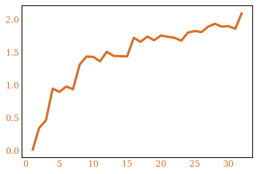
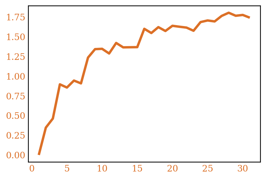
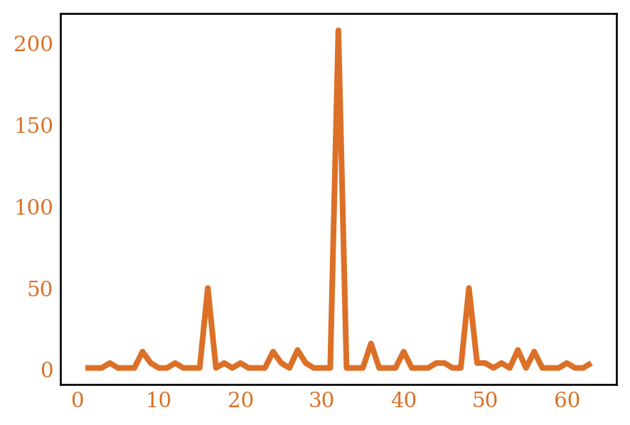
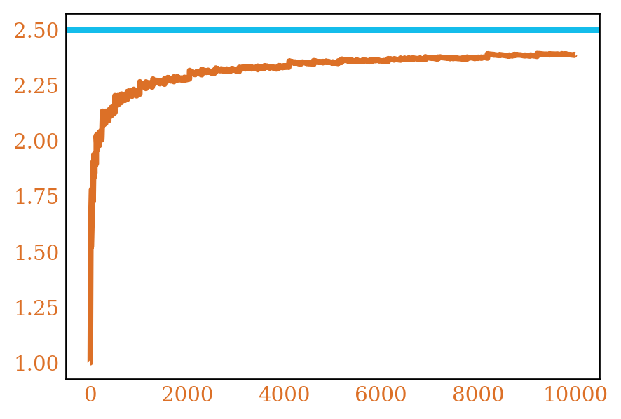
We can look at the average of \(\log f(n)\). Because \(f(n)\) is so fast growing, most of the terms in the average do not matter, so looking at \(\log f(n)\) might give some additional insight. This also means that \(f(n)\) acts like a polynomial so we could apply Dirichlet generating functions to this problem. We’ll do this implicitly, by invoking other results in analytic number theory. Figure 2 shows \(\frac{1}{x}\sum_{n \le x} \log f(n)\) computed for our ring counting functions.
For simplicity, let \(c = 1\) (this is a multiplicative constant that we can add in front later). In our case \(\log f(p^k) = k^3\log p\), and so \(\sum_{n \le x} \log f(n) = \sum_{n \le x} \sum_{i=1}^m k_i^3 \log p_i\). We can rearrange the sum by grouping prime powers: \(\sum_{p^k \le x} k^3 \log p |\{n \le x |\, p^k || n\}|\) The latter set’s cardinality is equal to \(\lfloor \frac{x}{p^k} \rfloor - \lfloor \frac{x}{p^{k+1}} \rfloor\), which is \(x (\frac{1}{p^k} - \frac{1}{p^{k+1}}) + O(1)\).
This lets us have \(\sum_{p^k \le x} k^3 \log p (x(\frac{1}{p^k} - \frac{1}{p^{k+1}}) + O(1)) = x\sum_{p^k \le x}k^3 \log p \frac{p - 1}{p^{k+1}} + O(\sum_{p^k \le x} k^3 \log p)\)
If we look at the latter sum inside the big-O, we can divide this into:
\(\sum_{p \le x} \log p + 2^3\sum_{p^2 \le x} \log p + 3^3 \sum_{p^3 \le x} \log p \ldots\). The first term is the second chebyshev function \(\psi(x)\). In fact we can write this series as
\(\sum_{k=1}^{\lfloor \log_2 x \rfloor} k^3 \psi(x^{\frac{1}{k}})\). As we have \(\psi(x) \sim x\) by the Prime Number Theorem, this series is asympotically \(x + O(\sqrt{x}(\log x)^4)\).
For the first term we have \(x\sum_{p^k \le x} k^3 \log p \frac{p-1}{p^{k+1}}\).
We can bound the latter term by an infinite sum \(\sum_p \sum_{k=1}^\infty k^3 \log p \frac{p-1}{p^{k+1}} = \sum_p \frac{p-1}{p}\log p\sum_{k=1}^\infty \frac{k^4}{p^{k}}\).
One can see that the inner sum is \(O(\frac{1}{p^2})\), and so the total sum will be bounded for some constant \(C\) by \(C\sum_p \frac{\log p}{p^2}\), which converges.
Thus we have \(\sum_{n \le x}\log f(n) = Mx + O(x) + O(\sqrt{x}(\log x)^4)\), so \(\frac{1}{x}\sum_{n\le x}\log f(n) = C + O(\frac{(\log x)^4}{\sqrt{x}})\), for some constant \(C\). In particular, for all our functions we have that \(\frac{1}{x}\sum_{n \le x} \log f(n)\) is bounded by some constant4
4 This is the best we can do since each of these functions \(\log f(n)\) has a \(O(k^{2.5}\log p)\) term that we have ignored. As this term can vary, and does contribute linearly in a similar way to the cubic term, we could theoretically produce two constants \(C_1\) and \(C_2\), for which the average fluctuates between.
Counting semisimple rings
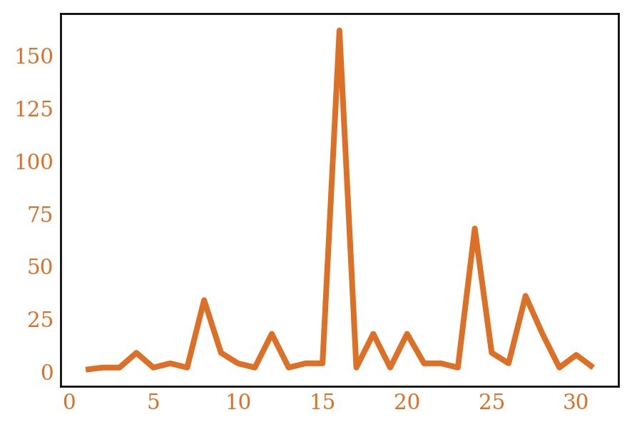
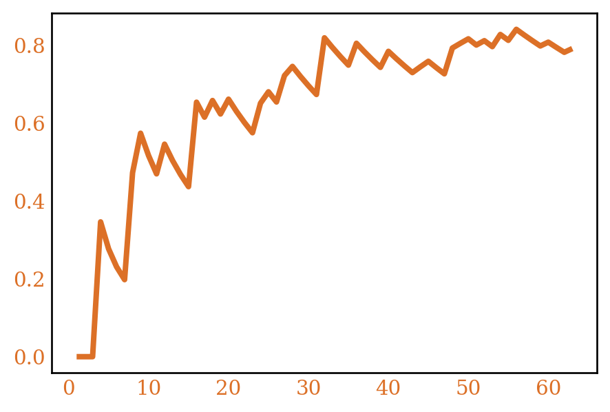
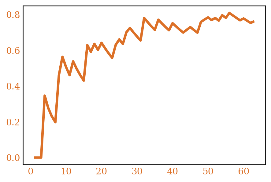
A semisimple ring \(R\) is one which is simple as a left \(R\)-module over itself. Let’s call the number of semisimple rings of order \(n\), \(r_*(n)\). Figure 3 plots \(r_*(n)\) and it’s average.
Semisimple rings are characterized by the Wedderburn-Artin theorem5, which says that a semisimple ring is one that is product of matrix algebras over skew fields.
5 See here for details.
In other words \(R = \prod_{i=1}^m M_{n_i \times n_i}(F_i)\). Because we are dealing with a finite ring \(R\), due to Wedderburn’s Little Theorem6, we have that \(F_i\) are actually all fields, and thus are order \(p_i^{r_i}\). The matrix algebra \(M_{n_i \times n_i}(F_i)\) then has the order \(p_i^{r_i^2}\). Let \(N_i\) bye the product of all \(M_{n_i \times n_i}(F_i)\) that are over fields of the same characteristic \(p\). Thus each factor \(N_i\) is a product over matrix rings over fields of different characteristics.
6 Wedderburn’s Little Theorem states that all finite skew-fields are fields. See here for details.
We’ll skip the details here, but this can be leveraged in a very similar way to the abelian group case to show that \(r_*(n)\) multiplicative.
Let’s look at \(r_*(p^k)\). Now \(R = \prod_{i=1}^m M_{n_i \times n_i}(F_i)\). Now all the \(F_i\) have to be fields of some prime order \(p^{k_i}\). This gives \(|M_{n_i \times n_i}(F_i)| = p^{k_i (n_i)^2}\), so that \(k = \sum_{i=1}^m k_i (n_i)^2\).
Again, we can leverage this like the abelian group case to get that \(r_*(p^k) = s(k)\), where \(s(k)\) is the number of ways to write \(k\) as a sum of ‘weighted’ squares \(k_i (n_i)^2\). For instance, \(r_*(p^4) = 5\) because \(4\) can be written as
\(1^2 + 1^2 + 1^2 + 1^2 \rightarrow M_{1\times 1}(\mathbb{F_p})^4\)
\((2)1^2 + 1^2 + 1^2 \rightarrow M_{1\times 1}(\mathbb{F_{p^2}}) \times M_{1 \times 1}(\mathbb{F_{p}})^2\)
\((2)1^2 + (2)1^2 \rightarrow M_{1 \times 1}(\mathbb{F_{p^2}})^2\)
\((3)1^2 + 1^2 \rightarrow M_{1 \times 1}(\mathbb{F_{p^3}}) \times M_{1 \times 1}(\mathbb{F_{p}})\)
\((4)1^2 \rightarrow M_{1 \times 1}(\mathbb{F_{p^4}})\)
\(2^2 \rightarrow M_{2\times 2}(\mathbb{F_{p}})\)
Forming the Dirichlet generating function \(f(s) = \sum_{n=1}^\infty \frac{r_*(n)}{n^s}\), we have the formal Euler product factorization into
\(f(s) = \prod_p \sum_{k=1}^\infty \frac{s(k)}{p^{ks}}\).
Let \(x = \frac{1}{p^s}\). Then \(\sum_{k=1}^\infty s(k)x^k\) is the generating function for \(s(k)\). Now the factor for a square is \((1 + x^{k^2} + x^{2k^2} + x^{3k^2} + \ldots x^{nk^2} \ldots) = \frac{1}{1 - x^{k^2}}\). This means the factor for a weighted square should be \(\frac{1}{1 - x^{lk^2}}\), where \(l \ge 1\).
Thus we get \(\sum_{k=1}^\infty s(k)x^k = \prod_{l=1}^\infty \prod_{k=1}^\infty \frac{1}{1 - x^{lk^2}}\) and so
\(f(s) = \prod_p \prod_{l=1}^\infty \prod_{k=1}^\infty \frac{1}{1 - (\frac{1}{p})^{lk^2s}} =\prod_{l=1}^\infty \prod_{k=1}^\infty \prod_p \frac{1}{1 - (\frac{1}{p})^{lk^2s}} = \prod_{l=1}^\infty\prod_{k=1}^\infty \zeta(lk^2s)\)7
7 We still have to prove absolute convergence, but it can be proven similar to the abelian group case to get convergence for \(\Re(s) > 1\).
8 The poles of this function will have a variety of orders. For instance, at \(\frac{1}{4}\) we have a pole of order 2, since \(\frac{1}{4} = \frac{1}{(1)2^2} = \frac{1}{(4)1^2}\).
Note that there are a lot of poles now. In particular, there is a pole at every \(\frac{1}{r^2 m}\), where \(r, m \in \mathbb{N}\). However, we will still have that the largest pole is simple at \(1\), followed by a simple pole at \(\frac{1}{2}\), which allows us to use a very similar contour as last time.8
Using the box contour from last time, we will get a contribution from the pole at \(1\), which gives a term of the form \(A x\), where \(A = \prod_{l=1, k=1, (l, k) \ne (1, 1)}^\infty \zeta(lk^2)\).
We won’t go through the analysis here 9, but proceeding as before will give \(\frac{1}{x}\sum_{n \le x} r_*(n) \sim A\).
9 The analysis is very simiilar to before, but there are more \(\zeta\) factors to contend with.