Counting the number of abelian groups

An asymptotic formula for the number of abelian groups

As an undergraduate, I got exposed to group theory and notably the classification of finite abelian groups ¹. I have recently thought about how to count asymptotically the number of these groups up to isomorphism. It turns out this problem was originally solved by Erdos and Szekeres², and we’’ll try to summarize an argument for the first order asymptotics here.

¹ And more generally the classification of finitely generated abelian groups.

² See here for their solution.

The main ideas of this proof are:

1. Establish that the function \(a(n)\) for the number of abelian groups of order \(n\) is multiplicative.
2. Write down a Dirchlet generating function for \(a(n)\) and show it has a very nice form.
3. Use tools of Complex Analysis (particularly Perron’s formula and the Cauchy residue theorem) to get a first order term.

Review: Whirlwind Group Theory

First, recall a group \(G\) is a set equipped with an operation \(*\), satisfying the following axioms:

1. Closure: \(a * b \in G,\, \forall a, b \in G\)
2. Associativity: \((a * b) * c = a * (b * c),\, \forall a, b, c \in G\)
3. Identity: \(\exists e \in G,\, \text{s.t.}\, \forall a \in G,\, e * a = a * e = a\)
4. Inverse: \(\forall a \in G,\, \exists a^{-1} \in G,\, \text{s.t.} \,a^{-1} * a = a * a^{-1} = e\)

A commutative group satisfies the following additional axiom

5. Commutativity: \(a * b = b * a,\, \forall a, b \in G\).

Since a group is a set \(G\), we can look at the cardinality of the set \(|G|\). A finite group is one where \(|G| < \infty\) and the order of a group is simply this number \(ord(G) = |G|\).

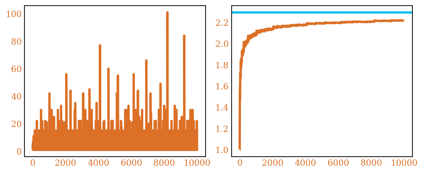
What we are interested in is how many finite abelian groups up to isomorphism have order \(n\). We’ll call this \(a(n)\). Figure 1 plots \(a(n)\) for orders 1 to 10000.

We can see that the number varies a lot, and unclear if it even grows. In particular if \(ord(G) = p\) for a prime \(p\), there is only one group of that order, \(\mathbb{Z}/p\mathbb{Z}\) the cyclic group of order \(p\). That is, \(a(p) = 1\) for all primes \(p\), so it dips to 1 infinitely often.

What we might care about instead is a smoothed version of this \(\frac{1}{x}\sum_{n \le x} a(n)\), which represents the average value of \(a(n)\). Figure 1 shows that this seems to be grow but asymptote around a little over \(2\). In fact as proven by Erdos and Szekeres we’ll have

\[\sum_{n \le x} a(n) \sim \prod_{k=2}^\infty \zeta(k) x\]

Where \(\zeta\) is the Riemann Zeta function. This constant in front is roughly \(2.29\), and is represented by the blue line in the plot.

Figure 1: Number of abelian groups of order N.

Number of Abelian Groups of order N

Structure of \(a(n)\).

The fundamental theorem of finite abelian groups says that every finite abelian group can be written in the form \(\mathbb{Z}/p_1^{k_1}\mathbb{Z} \times \mathbb{Z}/p_2^{k_2}\mathbb{Z} \times \mathbb{Z}/p_3^{k_3}\mathbb{Z} \ldots \mathbb{Z}/p_n^{k_n}\mathbb{Z}\) where \(p_i\) are primes, not necessarily distinct, and \(k_i \in \mathbb{N}\). ³

³ In fact each \(p_i\) must appear in the prime factorization of \(ord(G)\).

Recall that a finite \(p\)-group is which has prime power order \(ord(G) = p^k\) for some prime \(p\), and natural number \(k\).

We can group the factors into \(P_1, \ldots P_m\), where \(P_i\) is a product of factors containing the same prime. That is, every finite abelian group can be written as \(P_1 \times P_2 \times \ldots P_m\), where \(P_i\) are abelian \(q_i\)-groups, with the \(q_i\) distinct. The order of such a group \(G\) is \(ord(G) = ord(P_1)ord(P_2)\ldots ord(P_m)\).

This is suggestive that if we are looking at \(a(n)\), we should look at the prime factorization of \(n = p_1^{k_1}p_2^{k_2}\ldots p_m^{k_m}\). For any abelian group of order \(n\) it will have factors \(P_1 \times P_2 \ldots \times P_m\), where \(P_i\) is a \(p_i\)-group of order \(p_i^{k_i}\). Then, we will have \(a(n) = a(p_1^{k_1})a(p_2^{k_2})\ldots a(p_m^{k_m})\). In other words \(a(n)\) is a multiplicative function!

\(a(p^k)\)

Now, given a prime \(p\), we want to count the number of abelian groups of order \(p^k\), for some \(k \in \mathbb{N}\). We can enumerate a few cases to see a pattern.

For \(k = 1\), we have only one group, since \(\mathbb{Z}/p\mathbb{Z}\) is simple. \(a(p) = 1\)

For \(k = 2\) we have two groups: \(\mathbb{Z}/p^2\mathbb{Z}\) and \(\mathbb{Z}/p\mathbb{Z} \times \mathbb{Z} / p\mathbb{Z}\). \(a(p^2) = 2\)

For \(k = 3\) we have three groups: \(\mathbb{Z}/p^3\mathbb{Z}\), \(\mathbb{Z}/p^2\mathbb{Z} \times \mathbb{Z}/p\mathbb{Z}\) and \(\mathbb{Z}/p\mathbb{Z} \times \mathbb{Z}/p\mathbb{Z} \times \mathbb{Z}/p\mathbb{Z}\). \(a(p^3) = 3\)

What we’ve done above is take \(p^k\) and look at ways to partition \(k\).

For instance, the 11 partitions of \(6\) are:

1 + 1 + 1 + 1 + 1 + 1

2 + 1 + 1 + 1 + 1

2 + 2 + 1 + 1

3 + 1 + 1 + 1

2 + 2 + 2

3 + 2 + 1

4 + 1 + 1

3 + 3

4 + 2

5 + 1

6

We can then arrange factors based of that partition. If we take \([3, 2, 1]\), then we have \(\mathbb{Z}/p^3\mathbb{Z} \times \mathbb{Z}/p^2\mathbb{Z} \times \mathbb{Z}/p\mathbb{Z}\).

Likewise, given any factorization of the \(p\)-group, we can order the factors in descending order and show that forms a partition of \(6\). Thus, \(a(p^6) = 11\), and more generally \(a(p^k) = p(k)\) where \(p(k)\) is the number of partitions of \(k\).

Dirichlet Generating Function

Given that \(a(n)\) is a multiplicative function, it’s suggestive to look at \(f(s) = \sum_{i=1}^\infty \frac{a(n)}{n^s}\), at least formally. Since \(a(n)\) is multiplicative, it has an Euler product expansion \(f(s) = \prod_p \sum_{k=0}^\infty \frac{a(p^k)}{p^{sk}} = \prod_p \sum_{k=0}^\infty \frac{p(k)}{p^{sk}}\). It can be shown that the products converge for \(\Re(s) > 1\), due to the asymptotics of partition numbers \(p(k)\) (which we will skip here).

Now each inner sum is of the form \(\sum_{k=0}^\infty \frac{a(p^k)}{p^{sk}} = \sum_{k=0}^\infty \frac{p(k)}{p^{sk}}\). Let \(x = \frac{1}{p}\). Then we have the sum \(\sum_{k=0}^\infty p(k)x^{sk}\).

This is the ordinary generating function for the partition function, which also can be written as \(\prod_{k=1}^\infty \frac{1}{1 - x^{sk}}\). This is valid since \(\frac{1}{p} < 1\).

Thus we can rewrite \(f(n) = \prod_p \prod_{k=1}^\infty \frac{1}{1 - (\frac{1}{p})^{sk}}\). Applying the Fubini-Tonelli theorem⁴ lets us rearrange the product to get \(\prod_p \prod_{k=1}^\infty \frac{1}{1 - (\frac{1}{p})^{sk}} = \prod_{k=1}^\infty \prod_p \frac{1}{1 - (\frac{1}{p})^{sk}} = \prod_{k=1}^\infty \zeta(ks)\).

⁴ See here for a summary. In general, this will let us change the order of summation / multiplication.

⁵ We omit the proof of this here, but roughly the terms \(\zeta(ks) \rightarrow 1\) as \(k \rightarrow \infty\), and in fact this convergence is geometric in nature. We can then show that if we ignore the first few terms, in the strip \(\frac{1}{n+1} < \Re(s) < \frac{1}{n}\), the product converges, and will gives us a meromorphic continuation of the function.

Thus the Dirichlet generating function for \(a(n)\) is \(\prod_{k=1}^\infty \zeta(ks)\), which converges when \(\Re(s) > 1\). In fact we can meromorphically expand this to \(\Re(s) > 0\), by noting that there are poles at \(1, \frac{1}{2}, \frac{1}{3} \ldots \frac{1}{n} \ldots\), but the product still converges outside of those areas. ⁵

Counting the number of abelian groups

We’ve buried the lede so far on how we are going to estimate \(\sum_{n\le x} a(n)\). In particular, Perron’s Formula says that if \(f(s)\) is the Dirichlet generating function for \(a(n)\), then we have that if \(f(s)\) is uniformly convergent for \(\Re(s) > \sigma\) for some fixed \(\sigma\), and \(c > \sigma\), then⁶

⁶ For \(x\) an integer, we need to modify the sum so that the last term \(a(x)\) is multiplied by \(\frac{1}{2}\). Otherwise the left-hand side is an ordinary sum.

\[\sum_{n\le x} a(n) + O(\sum_{n=1}^\infty(\frac{x}{n})^c \frac{a(n)}{T|\log \frac{x}{n}|}) = \frac{1}{2\pi i} \int_{c-iT}^{c+iT} f(s)\frac{x^s}{s}ds\]

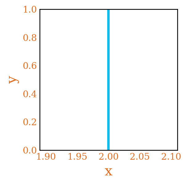
That is, if we we compute the line integral of the function \(A(s) = f(s)\frac{x^s}{s}\) over the truncated line \(\Re(s) = c\), that should give us what we want plus an error term. Figure 2 shows the contour for \(\Re(s) = 2\).

Figure 2: Contour for Perron’s Formula

Let’s bound the error term.

When \(n < 0.9x\) or \(n > 1.1x\) we have that

\(O(\sum (\frac{x}{n})^c \frac{a(n)}{T|\log \frac{x}{n}|}) = O(\frac{x^c}{T}\sum \frac{a(n)}{n^c}) = O(\frac{x^c\prod_{k=1}^\infty \zeta(kc)}{T}) = O(\frac{x\log x}{T})\).

The latter equality is a combination of three steps. We first fix \(c = 1 + \frac{1}{\log x}\) which gives us the linear power in \(x\). Also, noting that \(\prod_{k=2}^\infty \zeta(kc)\) is bounded, we only need to consider the \(\zeta(c)\) term. As \(\zeta(c) = O(\frac{1}{|c - 1|})\), for \(c\) approaching 1, the rest follows.

For \(0.9x \le n \le 1.1x\), \(O(\sum_{0.9x \le n \le 1.1x} (\frac{x}{n})^c \frac{a(n)}{T|\log \frac{x}{n}|}) = O(\sum_{0.9x \le n \le 1.1x} \frac{a(n)}{T|\log \frac{x}{n}|})\).

We’ll assume now that \(x = \lfloor x \rfloor + \frac{1}{2}\). That is, \(x\) is a half integer. Then, \(\frac{1}{|\log \frac{x}{n}|} = O(|\frac{x}{n - x - \frac{1}{2}}|)\), since \(n\) is close to \(x\).

If \(k = n - x\), we have our error bounded by \(O(\frac{x}{T}\sum_{|k| \le 0.1 x} \frac{1}{|k - \frac{1}{2}|}) = O(\frac{x\log x}{T})\) ⁷

⁷ The latter inequality comes from the fact that the Harmonic numbers grow like \(\log x\).

Modified Integral

We’ll modify the main integral by relating it to a shifted integral on the left hand size of the pole at 1.

Let \(c = 1 + \frac{1}{\log x}, \frac{1}{2} < \delta < 1\). Let \(A = \prod_{k=2}^\infty \zeta(k)\), and consider the contour in Figure 3, where we are integrating over it in the counterclockwise direction.

Figure 3: Modified Contour

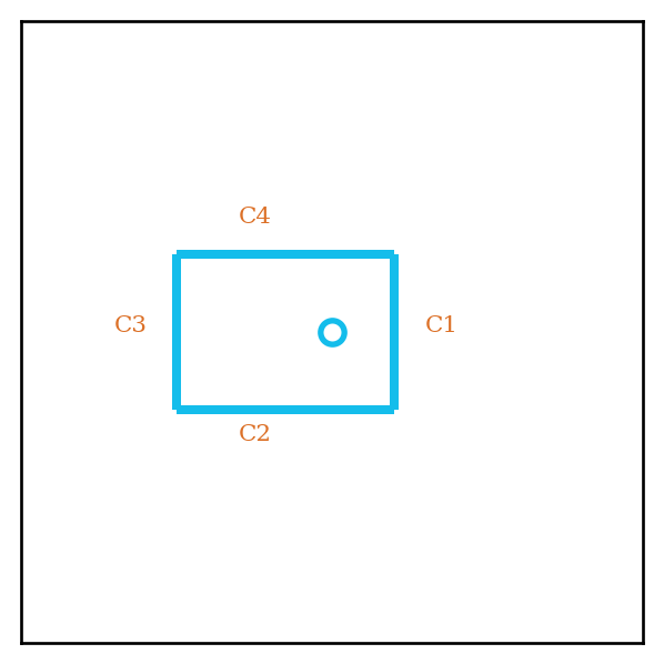
This contour \(B\) is now a box around the pole \(1\). \(C_1\) corresponds to our original contour (of length \(2T\)) while \(C_3\), is a shifted version.

We have the sides of the box parameterized as:

\(C_1 = \{s | \Re(s) = c, -T \le \Im(s) \le T\}\)

\(C_2 = \{s | \Im(s) = -T, \delta \le \Re(s) \le c\}\)

\(C_3 = \{s | \Re(s) = \delta, -T \le \Im(s) \le T\}\)

\(C_4 = \{s | \Im(s) = T, \delta \le \Re(s) \le c\}\)

Since \(\delta > \frac{1}{2}\), the box does not have any poles on its path, and only contains one pole inside. We have by the residue theorem, the value of this new contour is \(\frac{1}{2\pi i}\int_B f(s)\frac{x^s}{s} ds = Res_{s=1} f(s)\frac{x^s}{s} = \prod_{k=2}^\infty \zeta(k) x = Ax\)

Thus, breaking apart \(B\) into its constituent integrals, we get that \(Ax = \sum_{n\le x}a(n) + O(\frac{x\log x}{T}) + \int_{C_2 \cup C_3 \cup C_4} f(s)\frac{x^s}{s} ds\).

We will now bound the contours \(C_2, C_3, C_4\).

For \(C_2\), we can bound \(|f(s)|\) by \(B|\zeta(s)|\) where \(B = \prod_{k=2}^\infty \zeta(k\delta)\). This is due to the monotonicity of \(\zeta(s)\) for \(s > 1\), and that since \(\delta > \frac{1}{2}\), \(k\delta > 1, \, \forall k \ge 2\).

It is also known that \(|\zeta(s)| = O((1 + |\Im(s)|)^{1 - \Re(s)}\log(1 + \Im(s))\), for \(\Im(s) > 2, \Re(s) > 0\).

Thus, for \(C_2\) we have the bound \(|\int_{C_2} f(s)\frac{x^s}{s} ds| = O(\int_\delta^c |\zeta(s + iT)||\frac{x^{s + iT}}{s + iT}| ds) = O(\int_\delta^c \frac{x^s(1 + T)^{1 - s} \log T}{T} ds) = O(\frac{x\log x}{T} + \frac{x^\delta T^{1-\delta}\log T}{T})\) This same bound holds for \(C_4\) by a similar argument.

For \(C_3\) we have \(|\int_{C_3} f(s)\frac{x^s}{s} ds| = O(\int_{-T}^T|\zeta(\delta + iT)\frac{x^{\delta}}{\delta + it}| dt) = O(\int_{-T}^T(1 + |t|)^{1 - \delta}\frac{x^\delta}{1 + |t|}\log T dt) = O(x^\delta T^{1 - \delta}\log T)\)

Thus we have \(Ax = \sum_{n \le x} a(n) + O(\frac{x\log x}{T}) + O(\frac{x\log x}{T} + \frac{x^\delta T^{1-\delta}\log T}{T}) + O(x^\delta T^{1 - \delta}\log T)\)

Let \(\delta = \frac{1}{2} + \epsilon\), for \(\epsilon > 0\). Let \(T = \sqrt{x}\). Then we have the errors are of the form

\(O(\sqrt{x}\log x) + O(\sqrt{x} \log x + x^{\frac{1}{4} - \epsilon}\log x) + O(x^{\frac{1}{2} + \epsilon} x^{\frac{1}{4} - \frac{\epsilon}{2}}\log x) = O(x^{\frac{3}{4} + \epsilon})\).

The error is sublinear, and we are done.

More careful treatment can reduce this error down to \(O(\sqrt{x})\). In fact⁸ we have

⁸ See here for a summmary of asymptotics for this problem.

\[\sum_{n\le x} a(n) \sim Ax + B\sqrt{x} + Cx^{\frac{1}{3}} + O(x^{\frac{3}{10}}(\log x)^{\frac{9}{10}})\]

\(A = \prod_{k=1, k \ne 1}^\infty \zeta(k)\)

\(B = \prod_{k=1, k \ne 2}^\infty \zeta(\frac{k}{2})\)

\(C = \prod_{k=1, k \ne 3}^\infty \zeta(\frac{k}{3})\)

One can see that the constants \(B\) and \(C\) come from evaluating the residue of our integrand at the pole at \(\frac{1}{2}\) and at \(\frac{1}{3}\). The arguments get harder here with our tools because we will start accumulating more factors of \(\zeta(s)\) in the critical strip, which means we need tighter control of the growth rate of \(\zeta(s)\) in the strip.