1 Methods such as Clenshaw-Curtis or Gaussian Quadrature can do very well on smooth integrands with errors of \({\displaystyle O([2N]^{-k}/k)}\), where \(N\) is the number of quadrature points, and \(k\) is the number of derivatives \(f\) has.
Given a function \(f\) (we’ll assume \(f\) is \(C^\infty\) for simplicity, but some of these arguments can be changed depending on the smoothness) defined on the unit interval \([0, 1]\), we would like to compute the integral \(I = \int_0^1 f(x) dx\). Quadrature methods can easily deal with estimating these integrals 1
Our plan will be to come up with a lower variance (but biased) estimator, and then generalize to computing integrals of the form \(\int_A f(x) p(x) dx\), where \(p(x)\) is a probability density on some subset of \(\mathbb{R}\). Finally, we’ll be able to get an estimator even if we only have access to a sampler and the unnormalized log density (e.g. in the case of MCMC).
The typical Monte-Carlo estimator for this type of integral is \(S_n = \frac{1}{n}\sum_{i=1}^n f(u_i)\), where \(u_i \sim U(0, 1)\) are IID uniform samples. This is an unbiased estimator for \(I\) and has variance \(var(S_n) = \frac{var(f)}{n}\), where \(var(f)\) is the variance of the random variable \(f(U), U \sim U(0, 1)\). In particular the variance is inversely proportional to \(n\).
Trapezoid Rule Estimator
If we look at error estimates of various quadrature rules, we see that the errors get better dependency than \(O(\frac{1}{\sqrt n})\) for estimating \(I\).
We can see from the table that we can get errors \(S_n - I\) that are at least \(O(\frac{1}{n^2})\) for various Newton-Cotes formula. From wikipedia.
Name
Error Bound
Trapezoid Rule
\(-\frac{1}{12n^2}f''(\xi)\)
Simpson’s \(\frac{1}{3}\) rule Rule
\(-\frac{1}{90n^4}f^{(4)}(\xi)\)
Boole’s Rule
\(-\frac{8}{945n^6}f^{(6)}(\xi)\)
where \(\xi\) lies in the interval of integration \([a, b]\).
The main idea is we can exploit the structure of the trapezoid rule (and in general Newton-Cotes rules) to get better scaling of the variance with respect to the number of samples \(n\).
Given \(n\) samples \(u_i \sim U(0, 1)\), we can sort the samples to form the order statistics \(v_i\). We’ll also add the points \(0\) and \(1\) to get \(n + 1\) points (let \(v_0 = 0\) and \(v_{n + 1} = 1\)).
We can then consider the trapezoid rule estimator: \(S'_n = \sum_{i=0}^{n} \frac{1}{2} (v_{i+1} - v_i)(f(v_{i+1}) + f(v_i))\)
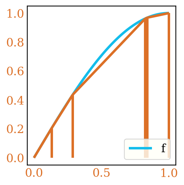
Figure 1: Randomized Trapezoid Rule for \(\sin(\frac{\pi}{2} x)\)
The intuition is that for sufficiently smooth \(f\), \(S'_n\) should be a good estimator of the integral \(I\) due to the use of the trapezoid rule. Note that \(S'_n\) may be biased, and indeed Figure 1 shows an example of this, where the trapezoid rule approximates the integral well, but will always be an underestimate due to the concavity of the integrand. The hope is that we may trade off some bias for a reduction in variance.
As mentioned above, we can note the following deficiencies of this method, compared to quadrature rules and monte carlo rules.
This can be a biased estimator.
This is for \(U(0, 1)\) random variables and in one dimension, for which there are better methods.
In the current formulation, you have to evaluate the endpoints \(0\) and \(1\). This can be problematic for integrands (such as certain \(Beta(\alpha, \beta)\) densities which go off to \(\infty\) in the tails). We can actually get away with \(n\) points without evaluating the \(0\) and \(1\) points. Adding the points just simplifies the analysis and reduces the error by a constant.
Error bound on \(S'_n\)
Let’s take a look at the error \(S'_n - I\).
For simplicity we’ll reuse a form of the Trapezoid Rule Error 2.
If we are estimating \(\int_{v_i}^{v_{i+1}} f(x) dx\), then the error of using \(\frac{1}{2}(f(v_{i+1}) + f(v_{i}))(v_{i+1} - v_i)\) is bounded by \(\frac{K_i(v_{i+1} - v_i)^3}{12}\), where \(K_i = \sup_{[v_i, v_{i+1}]} |f''(x)|\) (this can be derived through repeated applications of the Mean Value Theorem).
That is the \(k\)-th marginal moment grows like \(O(\frac{1}{n^k})\). and that the mixed moment \(\mathbb{E}[X_i^kX_j^k]\) grows like \(O(\frac{1}{n^{2k}})\).
We can look at \(\mathbb{E}[(S'_n - I)^2] = \mathbb{E}[(\frac{K}{12})^2 (\sum_{i=0}^{n + 1}(x_i)^3)^2]\) = \(\frac{K^2}{144}\sum_{i, j} \mathbb{E}[x_i^3x_j^3]\)
As the sum over the \((n + 2)^2\) terms is over moments which are all \(O(\frac{1}{n^6})\), this results in \(\mathbb{E}[(S'_n - I)^2)] = O(\frac{1}{n^4})\) (with an \(O(\frac{1}{n^2})\) bound on the bias) 4. A precise bound can be derived by carrying through the constants from the Trapezoid Rule and the Dirichlet moments.
4 One can easily get an error bound on the bias \(|\mathbb{E}[S'_n - I]|\) without squaring the sum. Mainly looking at \(\mathbb{E}[(S'_n - I)^2]\) gives us a stronger form of convergence, and one can still recover a bound on the bias.
Examples
Here’s some example on a few different functions on \([0, 1]\)
\(f = \frac{1}{1 + x^2}\)
\(g = e^x\sin(\frac{x}{2})\)
\(h = x^3 - x + x^2\).
Table 1: Absolute Error in estimating the integral of \(f = \frac{1}{1 + x^2}\), \(g = e^x \sin(\frac{x}{2})\), \(h = x^3 - x + x^2\).
Integral
Method
N=10
N=50
N=100
N=200
N=1000
0.785398
Monte Carlo
0.026491
0.019358
0.008144
0.002608
0.001540
0.785398
Trapezoid Rule
0.000393
0.000010
0.000038
0.000009
0.000000
0.785398
Simpson's 1/3 Rule
0.000002
0.000010
0.000001
0.000000
0.000000
Integral
Method
N=10
N=50
N=100
N=200
N=1000
0.488364
Monte Carlo
0.146778
0.003383
0.026795
0.034787
0.009164
0.488364
Trapezoid Rule
0.005188
0.000636
0.000118
0.000022
0.000001
0.488364
Simpson's 1/3 Rule
0.000131
0.000002
0.000000
0.000000
0.000000
Integral
Method
N=10
N=50
N=100
N=200
N=1000
0.083333
Monte Carlo
0.178741
0.057350
0.007101
0.011000
0.000868
0.083333
Trapezoid Rule
0.011265
0.001467
0.000173
0.000051
0.000002
0.083333
Simpson's 1/3 Rule
0.004317
0.000017
0.000001
0.000000
0.000000
We can see that the error of the estimates from the Trapezoid Monte Carlo estimator seem to decrease very rapidly.
“Improving” the Estimator
The above estimator can be extended to other Newton-Cotes-type estimators. A Newton-Cotes formula is an integration rule that estimates the integral via the integration of a polynomial interpolant on \(k + 1\) equally spaced points.
For instance, the trapezoid rule is just the integral of the linear polynomial between two equally spaced points.
For our purposes, we can take the interpolant and use it to derive an integration rule on non-qequally spaced points.
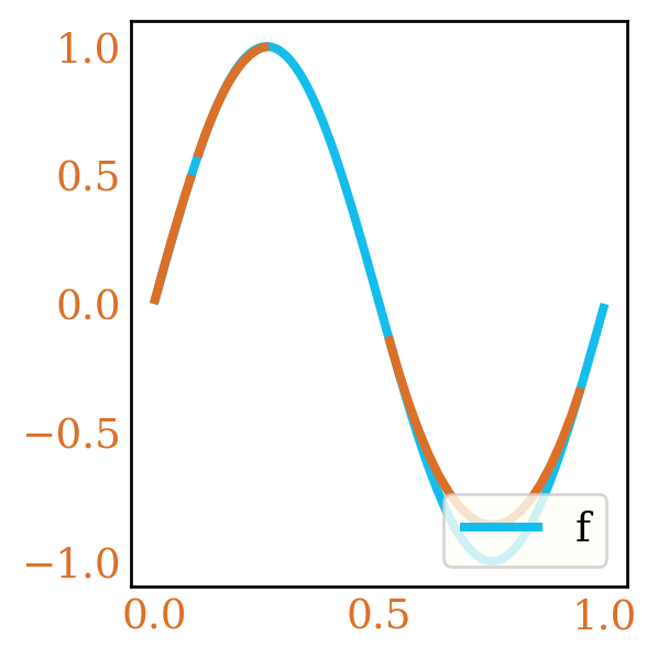
A Simpson’s Rule-type estimator, for instance would be of order 2 and use the \(3\) points next to each other (as seen in Figure 2).
Figure 2: Randomized Simpson Rule for \(\sin(2 \pi x)\)
The interpolating polynomial through the ordered points \(a, b, c\) would be \(p(x) = f(a)\frac{(c - x)(b - x)}{(c - a)(b - a)} + f(b)\frac{(c - x)(a - x)}{(c - b)(a - c)} + f(c)\frac{(a - x)(b - x)}{(a - c)(b - c)}\).
Error analysis for this can proceed in a similar way (though very messily), which should result in an estimator with \(\mathbb{E}[(S''_n - I)^2] = O(\frac{1}{n^8})\). Similary we should have a \(O(\frac{1}{n^4})\) bound on the bias.
In general, we can set up estimators from larger interpolating polynomials, to get asymptotically faster converging estimators 56.
5 Note that polynomial interpolation on equally spaced points can be very numerically unstable. These estimators defend against this by being on random points, but some care needs to be taken.
6 Note that while the Dirichlet moments will decay faster in \(n\) for higher order interpolants, they also pick up larger constants.
As seen in Table 1, we empirically get faster convergence with the Simpson’s-rule type estimator.
Extending to other probability distributions
Suppose now we have \(\int_{[a, b]} f(x) p(x) dx\), where \(p(x)\) is some probability density on some interval \([a, b]\)
The Monte Carlo estimate would be \(\sum_{i=0}^{n-1} f(x_i)\), where \(x_i \sim p(x)\). We would like to use our trapezoid estimator here, where we now have samples from \(p(x)\) rather than uniform samples.
We can naively apply the estimator by computing order statistics of \(x_i\), called \(z_i\), appending \(a\) and \(b\) to the ends much like before.
This gives the estimator \(S'_n = \sum_{i=0}^n \frac{1}{2}(z_{i+1} - z_i) (f(z_{i+1})p(z_{i+1}) - f(z_i)p(z_i))\)
Let \(v_i = F(z_i)\), where \(F\) is the CDF (we’ll assume this is completely differentiable). Then we have
Via an application of the Mean Value Theorem we have: \(S'_n = \sum_{i=0}^n \frac{1}{2}F'^{-1}(s_i) (v_{i+1} - v_i)(f(F^{-1}(v_{i+1}))p(F^{-1}(v_{i+1})) - f(F^{-1}(v_i))p(F^{-1}(v_i)))\)
for some \(s_i \in [v_i, v_{i+1}]\)
This suggests that if \(\sup_{[0, 1]} |F'^{-1}(u)| = \sup_{[a, b]} \frac{1}{p(x)} < \infty\), then we can pick up another constant and proceed with our error analysis as before, and thus get a \(O(\frac{1}{n^4})\) bound on \(\mathbb{E}[(I - S'_n)^2]\). More careful treatment in something like Phillipe (1997) can loosen this restriction.
We can apply this rule to a Beta density \(p(x)\) of a \(Beta(2, 3)\) random variable, with our functions from Table 1 to estimate \(\int_0^1 f(x)p(x) dx\).
Table 2: Absolute Error in estimating the integral of \(f = \frac{1}{1 + x^2}\), \(g = e^x \sin(\frac{x}{2})\), \(h = x^3 - x + x^2\) with respect to the Beta distribution.
Integral
Method
N=10
N=50
N=100
N=200
N=1000
0.849556
Monte Carlo
0.022431
0.015612
0.006972
0.006267
0.003704
0.849556
Trapezoid Rule
0.071244
0.004386
0.001175
0.003429
0.000172
0.849556
Simpson's 1/3 Rule
0.021684
0.000002
0.000070
0.000004
0.000000
Integral
Method
N=10
N=50
N=100
N=200
N=1000
0.331193
Monte Carlo
0.047922
0.032177
0.012697
0.005025
0.003999
0.331193
Trapezoid Rule
0.000814
0.001131
0.005256
0.001520
0.000146
0.331193
Simpson's 1/3 Rule
0.011204
0.000972
0.001880
0.001769
0.000013
Integral
Method
N=10
N=50
N=100
N=200
N=1000
-0.085714
Monte Carlo
0.061996
0.014922
0.000664
0.006580
0.001264
-0.085714
Trapezoid Rule
0.009933
0.001845
0.000278
0.000761
0.000123
-0.085714
Simpson's 1/3 Rule
0.015353
0.000206
0.001751
0.001618
0.000059
As seen in Table 2, we can still outperform the naive Monte-Carlo estimator.
If we only have access to an unnormalized density \(h(x)\), \(\frac{h(x)}{Z} = p(x)\), an application of Slutsky’s Theorem gives us the following estimator (where we simultaneously estimate the normalizing constant \(Z\)):
Thus, given a non-zero unnormalized density on \([a, b]\) and access to a sampler, we can estimate an expectation to any smooth function with this estimator 7.
7 In general we can mix and match estimators for the normalizing constant in the denominator. These estimators will be consistent, but in general will not be unbiased.
Other
This type of estimator seems to have been originally derived from Yakowitz and Szidarovszky (1978) for the unit interval. Phillipe (1997) and related works extend the Riemann sum estimator to other distributions.
Yakowitz, Krimmel, S., and F. Szidarovszky. 1978. “Weighted Monte Carlo Integration.”SIAM Journal on Numerical Analysis 15 (6): 1289–1300.
Phillipe, Anne. 1997. “Importance Sampling and Riemann Sums.”Publications IRMA Université de Lille 43 (IV).